7.6 - Points Along A Path¶

Hopefully you now have a basic understanding of how to move a camera. However, if you had to specify a unique position and orientation for a camera for every frame of an animation, which is typically running at 30 frames per second, you have a lot of work ahead of you!

Animations have a concept called keyframing. To use keyframing you assign a starting position and orientation to a camera (or any obect) for a particular frame. Then you assign an ending position and orientation for a future frame. Then the computer calculates the position and orientation of the camera for each intermediate frame. Keyframing is fundamental to all 3D computer graphics animations.

This lesson describes how to calculate intermediate values between a starting and ending value.

Parametric Equations¶

Given a starting and ending value, we want to calculate intermediate values between them. We assume we know the time (or frame) of the starting value and the time (or frame) of the ending value. Parametric equations are the ideal method for these calculations. A parametric equation is a function of a single variable, which we usually call t. Think of t as representing time. To be as generic as possible we assume that t varies between 0.0 and 1.0. You can always scale the results to match any particular time interval.

Let’s start off with a simple example. Let’s calculate points along a straight line between two points, p1 and p2. All intermediate points between p1 and p2 can be calculated using a fractional combination of the two points. The equation looks like this:

p = (1-t)*p1 + t*p2;  // where t varies from 0.0 to 1.0

Notice the following:

When t = 0.0, the equation becomes p = p1.
When t = 1.0, the equation becomes p = p2.
When t = 0.25, the equation becomes p = 0.75*p1 + 0.25*p2. The point p is 25% away from p1 and 75% away from p2.
t + (1-t) is always equal to 1.0. This means we are always getting 100% of the two points. For any value of t, you are taking t% of p2 and the leftover percentage of p1.
For a straight line in 3D space, we are calculating 3 values but only varying a single parameter t:
- p_x = (1-t)*p1_x + t*p2_x
- p_y = (1-t)*p1_y + t*p2_y
- p_z = (1-t)*p1_z + t*p2_z

All of the parametric equations we will discuss take a percentage of the original values to produce intermediate values. it is a really simple and elegant idea.

Basis Functions¶

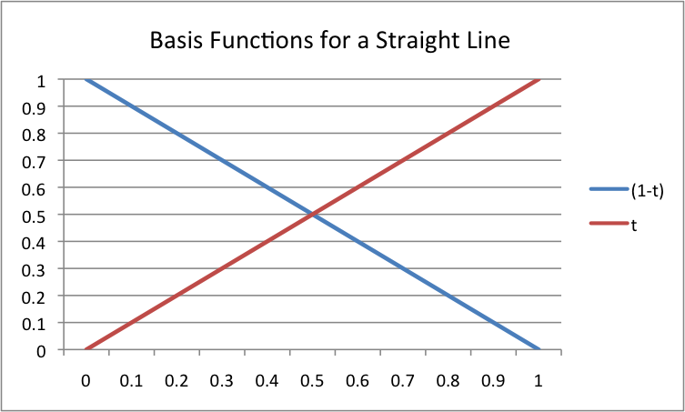
The functions that produce the fractions used for a parametric equation are called basis functions . Let’s plot the basis functions for the simple example above. The basis functions are (1-t) and (t). A plot of these two functions for values of t between 0.0 and 1.0 gives the straight lines in the diagram. Please notice the following about these basis functions:

Every value for t is a fraction. The t values are percentages.
When t=0, (1-t) is one and (t) is zero. This forces the equation to calculate p1 when t=0.
The basis functions are linear, which makes the intermediate points lie on a straight line.
The basis functions sum to one for all values of t. If this property is true for a set of basis functions, then all of the intermediate points on a path lie inside the convex hull of the points that define the path.

It is beyond the scope of these tutorials to delve into all the possibilities for basis functions, but perhaps you can get the big idea and pursue more information about parametric equations at a future time. Here is the “big idea”:

The Big Idea

A continuous path can be defined by a series of points. The basis functions that are used to combine percentages of the points determines the exact path.

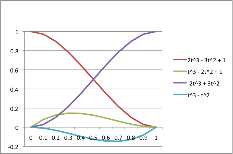
Here is an example to “wet you appetite”. Given four points you can calculate intermediate points along a curve that approximates these points using percentages of the four points calculated like this:

p = (2t³ - 3t² + 1)*p1 + (t³ - 2t² + t)*p2 + (-2t³ + 3t²)*p3 + (t³ - t²) p4

A plot of the basis functions is shown to the right. There are many possible basis functions that will calculate paths through a series of points. Perhaps you will have an interest to pursue these ideas deeper at a later time.

Circular Paths¶

Calculating intermediate points around a circular path that is centered about an arbitrary 3D point and about an arbitrary rotation vector is best done with a matrix transformation. Since all rotation is about the origin, you need to do the following three steps:

Translate the center point to the global origin.
Use a rotation transform to rotate about the axis of rotation.
Translate the center point back to its original position.

As in the parametric equation case, you are using a single value to calculate a new location along a path, but in this case the single value is an angle.

Glossary¶

keyframing: Set the position and orientation of an object at key frames and have the computer calculate the position and orientation of the object at intermediate frames.
parametric equations: Calculate intermediate points along a path defined by a series of points. Any particular intermediate point is defined by a single parameter t.
basis functions: A set of functions that calculate the percentage of contribution a point has to the location of an intermediate point.

Next Section - 7.7 - Timing Along A Path