7.7 - Timing Along A Path¶

Let’s assume you are using a parametric equation to change the position and orientation of an object over a series of frames for an animation. The value of the parametric parameter t needs to vary from 0.0 to 1.0 over the frames that contain the movement. This lesson discusses how to calculate appropriate values for t.

Speed and Acceleration¶

Speed is defined as distance divided by time. For cars we use miles/hour; for a person running, perhaps meters/second. Distance, time, and speed are interrelated using these basic formulas:

speed = distance / time;
distance = speed * time;
time = distance / speed;

When you are designing an animation you have to chose two of the three values and the third value “is what it is.” So you have 3 scenarios for designing an animation:

You decide the distance to travel and the time of travel.
You decide the speed of movement and the time of travel.
You decide the distance of travel and the speed.

Option 1 is perhaps the most common and that is what we will discuss in this lesson.

For an animation you can measure time in seconds or in frames. Distance can be measured using any units that are consistent with your virtual scene. Remember that WebGL is unit-less; you just need to use consistent units for all measurements.

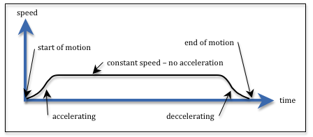
Acceleration is the change in speed over time. When you are accelerating you are increasing your speed. When you are decelerating you are decreasing your speed. In the real world you can’t instantaneously start traveling at a particular speed, nor can you stop instantaneously. Any object that starts to move must accelerate to a given speed, travel at that speed for a certain amount of time, and then decelerate until the object is stationary. This is visualized in the diagram.

We often make simplifying assumptions about motion when we create virtual worlds. Let’s consider two scenarios:

We ignore acceleration entirely.
We include acceleration, but model it as a linear change.

Ignore Acceleration¶

For simple motion it is sometimes acceptable to ignore acceleration and immediately start moving at a constant speed. For the parametric parameter t, if the difference between your values of t are equal, your change in locations will be a constant distance, which means you will be moving at a constant speed. To calculate your “change in t” for such a motion, simply calculate the number of discrete positions an object will have during the motion. Then divide this into 1.0, since t varies between 0.0 and 1.0. (Note that given n frames, there are (n-1) transitions between frames.)

number_frames = ending_frame - starting_frame + 1;
dt = 1.0 / (number_frames-1);

Let’s walk through a specific example. In frame 100 an object is stationary and has a location of p1 = (10, 12,-4). You want the object to move to location p2 = (20, 8, 5) by frame 110. In frames 101 through 109 the object will be in a location calculated by the parametric equation. Using the above equations the values for dt is 0.1 and the values for t for each frame will be:

frame number	100	101	102	103	104	105	106	107	108	109	110
frame number	100	101	102	103	104	105	106	107	108	109	110
dt =		0.100	0.100	0.100	0.100	0.100	0.100	0.100	0.100	0.100	0.100
dt =		0.100	0.100	0.100	0.100	0.100	0.100	0.100	0.100	0.100	0.100
t =	0.000	0.100	0.200	0.300	0.400	0.500	0.600	0.700	0.800	0.900	1.000
t =	0.000	0.100	0.200	0.300	0.400	0.500	0.600	0.700	0.800	0.900	1.000
	start	constant speed									end

The selection of the starting and ending frames determines the time for the animation. You can convert the number of frames into seconds by dividing by the frame rate. For example:

seconds = (number_frames-1) / (30 frames/ 1 sec);

The selection of the starting and ending points determines the distance of the motion. You could calculate the exact distance using the distance formula:

distance = Math.sqrt( (p2x-p1x)*(p2x-p1x) + (p2y-p1y)*(p2y-p1y) + (p2z-p1z)*(p2z-p1z));

If we needed the exact speed of the motion we could calculate it:

speed = distance / seconds;

Include Acceleration¶

For more realistic motion you need to include the acceleration of the object as it starts to move and the deceleration as it slows down to stop. This adds complexity to your animation design and to your calculations.

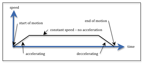
To simplify our calculations as much as possible we consider the acceleration and deceleration to be linear functions as shown in the diagram. There are many scenarios we could consider, but let’s look at a straightforward one where the animation designer decides the time it takes to accelerate and decelerate. The equations will be developed using the simple example we used above: in frame 100 an object is stationary and has a location of p1 = (10, 12,-4); you want the object to move to location p2 = (20, 8, 5) by frame 110; and acceleration takes 3 frames at the beginning of the motion and deceleration takes 2 frames at the end of the motion. The table below lays out the scenario with the values we need to calculate. Please note that we need to calculate the “change in t” between frames in order to calculate the the actual values of t. We will end up with 11 values for t, but 10 “change in t” values.

frame number	100	101	102	103	104	105	106	107	108	109	110
frame number	100	101	102	103	104	105	106	107	108	109	110
dt =		?	?	?	dt	dt	dt	dt	dt	?	?
dt =		?	?	?	dt	dt	dt	dt	dt	?	?
t =	0.000	?	?	?	?	?	?	?	?	?	1.00
t =	0.000	?	?	?	?	?	?	?	?	?	1.00
	accelerating				constant speed					decelerating
	accelerating				constant speed					decelerating

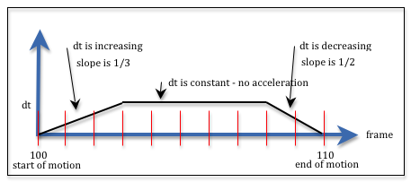
Let’s call the “change in t” dt. If dt is constant, then we have constant speed. If dt is increasing we have acceleration; if dt is decreasing we have deceleration. We use the slope of the acceleration and deceleration lines to approximate the dt value at the start and end of the motion. We don’t know the value for dt but we do know that the sum of all the values must be 1.0. For the specific example in the diagram, we can write the equation below. In the diagram the frames are marked with vertical red lines. Notice that we take the value for dt in the middle of each frame.

// Adding the dt values for acceleration, constant speed, and deceleration
1.0 = 1/6*dt + 3/6*dt + 5/6*dt + dt + dt + dt + dt + dt + 3/4*dt + 1/4*dt;

Therefore 7.5*dt === 1.0 and dt must be 1/7.5, or 0.133. Substituting this value for dt back into each term gives us the specific “change in t” for each frame. These values are show in the following table.

frame number	100	101	102	103	104	105	106	107	108	109	110
frame number	100	101	102	103	104	105	106	107	108	109	110
dt =	0.000	0.022	0.067	0.111	0.133	0.133	0.133	0.133	0.133	0.100	0.033
dt =	0.000	0.022	0.067	0.111	0.133	0.133	0.133	0.133	0.133	0.100	0.033
t =	0.000	0.022	0.088	0.200	0.333	0.467	0.600	0.733	0.866	0.966	1.000
t =	0.000	0.022	0.088	0.200	0.333	0.467	0.600	0.733	0.866	0.966	1.000
	accelerating				constant speed					decelerating
	accelerating				constant speed					decelerating

Let’s make some observations about the calculated values:

For this problem the dt value is 0.133, while for the original “constant speed” problem above the dt value was 0.1. It makes sense that the speed during constant motion must be greater to make up for the time lost during acceleration and deceleration.
The dt values are increasing during acceleration and decreasing during deceleration. Hopefully this makes sense from a physical perspective as well.

With a little work we can generalize this algorithm for any set of inputs. The function calculateAnimation in the demo code below will calculate and return an array of t values based on a starting frame, an ending frame, the number of frames to accelerate, and the number of frames to decelerate. Please study the code carefully. Then experiment with the WebGL demo program.

Show: Code Canvas Run Info

path.js

/**
 * path.js, By Wayne Brown, Spring 2016
 */

/**
 * The MIT License (MIT)
 *
 * Copyright (c) 2015 C. Wayne Brown
 *
 * Permission is hereby granted, free of charge, to any person obtaining a copy
 * of this software and associated documentation files (the "Software"), to deal
 * in the Software without restriction, including without limitation the rights
 * to use, copy, modify, merge, publish, distribute, sublicense, and/or sell
 * copies of the Software, and to permit persons to whom the Software is
 * furnished to do so, subject to the following conditions:
 *
 * The above copyright notice and this permission notice shall be included in all
 * copies or substantial portions of the Software.

* THE SOFTWARE IS PROVIDED "AS IS", WITHOUT WARRANTY OF ANY KIND, EXPRESS OR
 * IMPLIED, INCLUDING BUT NOT LIMITED TO THE WARRANTIES OF MERCHANTABILITY,
 * FITNESS FOR A PARTICULAR PURPOSE AND NONINFRINGEMENT. IN NO EVENT SHALL THE
 * AUTHORS OR COPYRIGHT HOLDERS BE LIABLE FOR ANY CLAIM, DAMAGES OR OTHER
 * LIABILITY, WHETHER IN AN ACTION OF CONTRACT, TORT OR OTHERWISE, ARISING FROM,
 * OUT OF OR IN CONNECTION WITH THE SOFTWARE OR THE USE OR OTHER DEALINGS IN THE
 * SOFTWARE.
 */

"use strict";
var Learn_webgl_matrix, Learn_webgl_vector3, Learn_webgl_point3;

//-----------------------------------------------------------------------
/**
 * Store and manipulate a path between two points.
 * @param scene PointsAlongAPathRender
 * @param x1 Number The x component for P1
 * @param y1 Number The y component for P1
 * @param z1 Number The z component for P1
 * @param x2 Number The x component for P2
 * @param y2 Number The y component for P2
 * @param z2 Number The z component for P2
 * @constructor
 */
window.Path = function (scene, x1, y1, z1, x2, y2, z2) {

// Constructor
  var self = this;

// Objects needed for internal elements and calculations
  var P = new Learn_webgl_point3();

// The points that define the path
  self.P1 = P.create(x1, y1, z1);
  self.P2 = P.create(x2, y2, z2);
  self.animate_active = false;

// Scratch objects for calculations
  var p;
  p = P.create();  // an intermediate point along the path

var previous_time = 0;
  var frame_rate = 16; // 1/60 of a second in milliseconds
  var frame_index = 0;
  var max_frame = 0;
  var ts = [];

//-----------------------------------------------------------------------
  /**
   * Calculate an intermediate point along a straight path between P1 and P2.
   * @param t
   */
  self.intermediatePoint = function (t) {

p[0] = (1 - t) * self.P1[0] + t * self.P2[0];
    p[1] = (1 - t) * self.P1[1] + t * self.P2[1];
    p[2] = (1 - t) * self.P1[2] + t * self.P2[2];

return p;
  };

//-----------------------------------------------------------------------
  /**
   * Calculate the values of t needed for a path between P1 and P2
   * @param starting_frame Number The frame to start the animation
   * @param ending_frame Number The frame to end the animation
   * @param frames_for_acceleration Number The number of frames before constant speed
   * @param frames_for_deceleration Number The number of frames after constant speed
   */
  self.calculateAnimation = function (starting_frame, ending_frame,
                                      frames_for_acceleration,
                                      frames_for_deceleration) {
    var number_frames, dt, j, k, n, sum, slope, constant;

// Allocate an array for the parametric t values
    number_frames = ending_frame - starting_frame + 1;
    ts = new Array(number_frames);

// How many frames have constant speeds?
    constant = (number_frames - 1) - frames_for_acceleration - frames_for_deceleration;

frame_index = 0;
    max_frame = number_frames;

if (constant < 0 ||
        (frames_for_acceleration === 0 && frames_for_deceleration === 0)) {
      // Constant speed for each step
      dt = 1.0 / (number_frames - 1);

// Fill the array
      for (j = 0; j < number_frames; j += 1) {
        ts[j] = dt * j;
      }
    } else {
      // Add up the acceleration step changes
      sum = 0;
      slope = frames_for_acceleration * 2;
      for (j = 0, k = 1; j < frames_for_acceleration; j += 1, k += 2) {
        sum += k / slope;
      }

// Add in the frames with constant speed
      sum += constant;

// Add up the deceleration step changes
      slope = frames_for_deceleration * 2;
      for (j = 0, k = 1; j < frames_for_deceleration; j += 1, k += 2) {
        sum += k / slope;
      }

// Calculate the dt needed for the constant speed section
      dt = 1.0 / sum;

ts[0] = 0;
      n = 1;
      // Fill in the acceleration deltas
      slope = frames_for_acceleration * 2;
      for (j = 0, k = 1; j < frames_for_acceleration; j += 1, k += 2, n += 1) {
        ts[n] = ts[n - 1] + (k / slope) * dt;
      }

// Fill in the constant speed deltas
      for (j = 0; j < constant; j += 1, n += 1) {
        ts[n] = ts[n - 1] + dt;
      }

// Fill in the acceleration deltas
      slope = frames_for_deceleration * 2;
      for (j = 0, k = slope - 1; j < frames_for_deceleration; j += 1, k -= 2, n += 1) {
        ts[n] = ts[n - 1] + (k / slope) * dt;
      }

}
  };

//-----------------------------------------------------------------------
  /**
   * Animate an object for every location along the path between P1 and P2.
   */
  self.animate = function () {
    var now, elapsed_time;

if (self.animate_active) {

now = Date.now();
      elapsed_time = now - previous_time;

if (elapsed_time >= frame_rate) {

if (frame_index < max_frame) {
          scene.t = ts[frame_index];
          frame_index += 1;
          scene.render();
          scene.events.updateValuesDisplay();
        } else {
          self.animate_active = false;
          return;
        }

// Remember when this scene was rendered.
        previous_time = now;
      }

window.requestAnimationFrame(self.animate);
    }
  };
};

To investigate linear motion between two points, P1 and P2:

Manipulate the location of the two points.
Select whether you want to include acceleration.
Set the number of frames for the animation.
Set the number of frames to use for acceleration and deceleration.
Push the Animate button to animate a small sphere between the P1 and P2

Click the Animate button to move between P1 and P2.

P1 (5.0, 0.0, 0.0)	P2 (-5.0, 0.0, 0.0)	t = 0.0
X: -5.0 +5.0	X: -5.0 +5.0
Y: -5.0 +5.0	Y: -5.0 +5.0	t: 0.0 +1.0
Z: -5.0 +5.0	Z: -5.0 +5.0

No acceleration, only constant speed.
Include acceleration and deceleration.
2 150    Number of frames: 30
0 50    Frames for acceleration: 0
0 50    Frames for deceleration: 0

Shader errors, Shader warnings, Javascript info

Open this webgl program in a new tab or window

Summary¶

You can change an object’s location, orientation, and possibly other properties by using parametric equations which use a single input, t, to specify intermediate values. If we vary t correctly, we can simulate acceleration, constant speed, and deceleration. There are three major scenarios for calculating the values of t, based on whether you specify distance and time, which requires calculating speed, or you specify distance and speed, which requires calculating time, or you specify speed and time, which requires calculating distance. In the above examples we specified distance and time, which required that we calculate speed (which was the dt values). There are many other possible scenarios than the two we have discussed here.

Glossary¶

speed: The rate of change in an object’s location and/or orientation, measured in terms of distance per change in time.
acceleration: The change in speed over a time interval.

Next Section - 7.8 - Screen Updates and Animation